Meudon PDR code emulator predictions
This notebook shows how to use the MeudonPDR class, which provides a fast, memory-light and accurate emulator of the Meudon PDR code.
[1]:
import os
import sys

import matplotlib.pyplot as plt
import pandas as pd

sys.path.insert(0, os.path.join(".."))

from infobs.model import MeudonPDR
from infobs.graphics import PDRPlotter

%load_ext autoreload
%autoreload 2
Predictions from a grid of parameters
[2]:
lines = ["13c_o_j1__j0", "13c_o_j2__j1", "13c_o_j3__j2"]
Grid setup
[3]:
df_params = pd.DataFrame(
    {
        "Av": [1, 5, 10, 15, 20],
        "G0": [1e2, 1e2, 1e2, 1e2, 1e2],
        "Pth": [1e5, 1e5, 1e5, 1e5, 1e5],
        "angle": [0, 0, 0, 0, 0],
    }
)

df_params
[3]:
| Av | G0 | Pth | angle | |
|---|---|---|---|---|
| 0 | 1 | 100.0 | 100000.0 | 0 |
| 1 | 5 | 100.0 | 100000.0 | 0 |
| 2 | 10 | 100.0 | 100000.0 | 0 |
| 3 | 15 | 100.0 | 100000.0 | 0 |
| 4 | 20 | 100.0 | 100000.0 | 0 |
Predictions of integrated line intensities
[4]:
meudonpdr = MeudonPDR()
meudonpdr.predict(df_params, lines)
[4]:
| Av | G0 | Pth | angle | kappa | 13c_o_j1__j0 | 13c_o_j2__j1 | 13c_o_j3__j2 | |
|---|---|---|---|---|---|---|---|---|
| 0 | 1.0 | 100.0 | 100000.0 | 0.0 | 1.0 | 0.000276 | 0.000318 | 0.000128 |
| 1 | 5.0 | 100.0 | 100000.0 | 0.0 | 1.0 | 10.176692 | 11.708745 | 3.919423 |
| 2 | 10.0 | 100.0 | 100000.0 | 0.0 | 1.0 | 22.873276 | 21.915024 | 8.102161 |
| 3 | 15.0 | 100.0 | 100000.0 | 0.0 | 1.0 | 29.498773 | 25.964494 | 10.321277 |
| 4 | 20.0 | 100.0 | 100000.0 | 0.0 | 1.0 | 34.912525 | 29.605632 | 12.635616 |
Integrated intensity unit
Set the kelvin parameter to False if you want integrated line intensities in erg cm-2 s-1 sr-1
[5]:
meudonpdr = MeudonPDR(kelvin=False)
meudonpdr.predict(df_params, lines)
[5]:
| Av | G0 | Pth | angle | kappa | 13c_o_j1__j0 | 13c_o_j2__j1 | 13c_o_j3__j2 | |
|---|---|---|---|---|---|---|---|---|
| 0 | 1.0 | 100.0 | 100000.0 | 0.0 | 1.0 | 3.785540e-13 | 3.483762e-12 | 4.746177e-12 |
| 1 | 5.0 | 100.0 | 100000.0 | 0.0 | 1.0 | 1.395919e-08 | 1.284490e-07 | 1.451301e-07 |
| 2 | 10.0 | 100.0 | 100000.0 | 0.0 | 1.0 | 3.137487e-08 | 2.404155e-07 | 3.000103e-07 |
| 3 | 15.0 | 100.0 | 100000.0 | 0.0 | 1.0 | 4.046295e-08 | 2.848396e-07 | 3.821807e-07 |
| 4 | 20.0 | 100.0 | 100000.0 | 0.0 | 1.0 | 4.788890e-08 | 3.247841e-07 | 4.678770e-07 |
Adding a scaling parameter to integrate uncertainty on geometry and beam dilution
In this example, we assume the logarithm of the scaling parameter \(\kappa\) to be uniformly distributed:
When not specified, the kappa parameter is constant equal to 1 and therefore has no impact.
While the predictions of the PDR code emulator are deterministic, adding this parameter to the model introduces randomness. This parameter is sampled from a Sampler, see the samplers.ipynb notebook for more details.
[6]:
from infobs.sampling import LogUniform

kappa = LogUniform(10**-0.5, 10**0.5)

meudonpdr.predict(df_params, lines, kappa=kappa)
[6]:
| Av | G0 | Pth | angle | kappa | 13c_o_j1__j0 | 13c_o_j2__j1 | 13c_o_j3__j2 | |
|---|---|---|---|---|---|---|---|---|
| 0 | 1.0 | 100.0 | 100000.0 | 0.0 | 0.362598 | 1.372631e-13 | 1.263207e-12 | 1.720956e-12 |
| 1 | 5.0 | 100.0 | 100000.0 | 0.0 | 1.245769 | 1.738993e-08 | 1.600178e-07 | 1.807985e-07 |
| 2 | 10.0 | 100.0 | 100000.0 | 0.0 | 1.030183 | 3.232187e-08 | 2.476720e-07 | 3.090656e-07 |
| 3 | 15.0 | 100.0 | 100000.0 | 0.0 | 2.247830 | 9.095385e-08 | 6.402709e-07 | 8.590772e-07 |
| 4 | 20.0 | 100.0 | 100000.0 | 0.0 | 0.408667 | 1.957059e-08 | 1.327284e-07 | 1.912057e-07 |
Prediction plots
[7]:
plotter = PDRPlotter(kelvin=True)
plotter.print_parameters_space()
Parameters space
Av: [1, 40] mag
G0: [0.6393, 63930.0]
Pth: [100000.0, 1000000000.0] K.cm-3
angle: [0, 60] deg
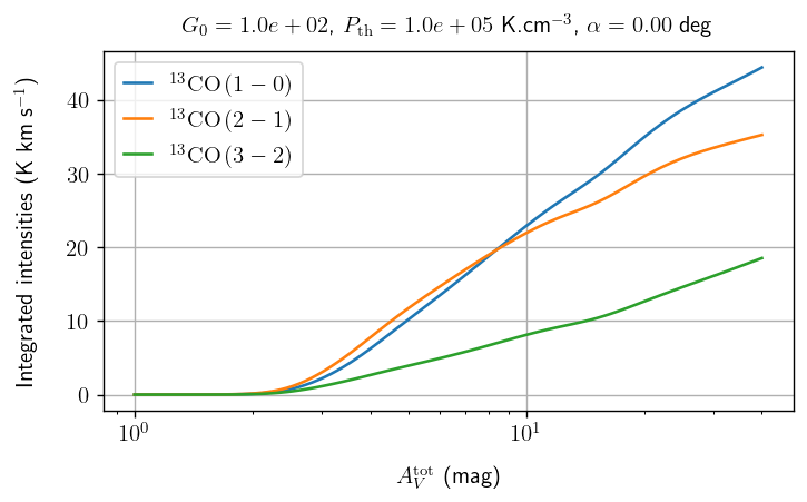
Profiles
[8]:
lines = ["13c_o_j1__j0", "13c_o_j2__j1", "13c_o_j3__j2"]

Av = 6
G0 = 1e2
Pth = 1e5
[9]:
plt.figure(figsize=(6.4, 0.7 * 4.8), dpi=125)

plotter.plot_profile(
    lines,
    Av=None,
    G0=1e2,
    Pth=1e5,
    angle=0,
    logy=False,
)

plt.show()
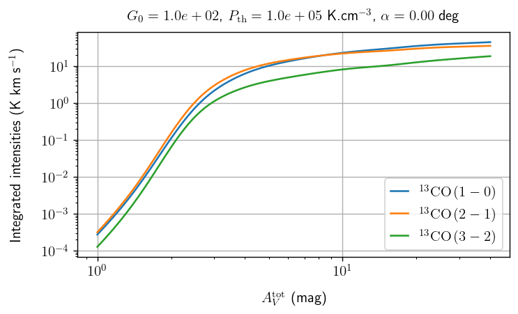
[10]:
plt.figure(figsize=(6.4, 0.7 * 4.8), dpi=125)

plotter.plot_profile(
    lines,
    Av=None,
    G0=1e2,
    Pth=1e5,
    angle=0,
    logy=True,
)

plt.show()
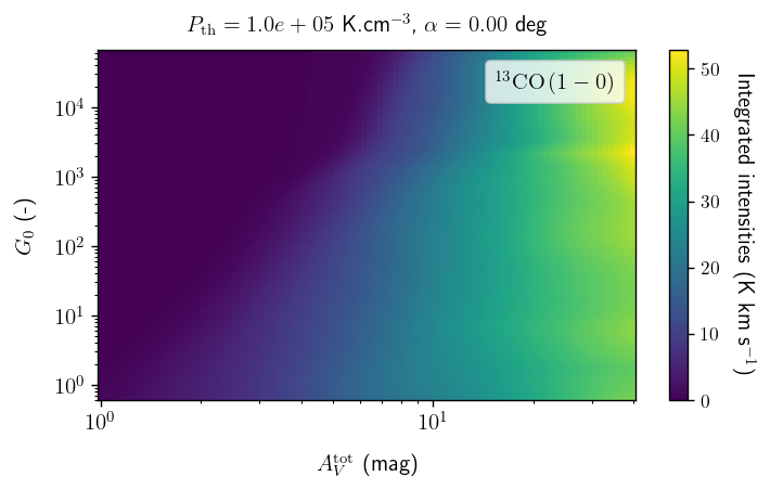
Slice (color plot)
[11]:
line = "13c_o_j1__j0"
[12]:
plt.figure(figsize=(6.4, 0.7 * 4.8), dpi=125)

plotter.plot_slice(
    line,
    Av=None,
    G0=None,
    Pth=1e5,
    angle=0,
    logz=False,
)

plt.show()
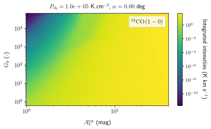
[13]:
plt.figure(figsize=(6.4, 0.7 * 4.8), dpi=125)

plotter.plot_slice(
    line,
    Av=None,
    G0=None,
    Pth=1e5,
    angle=0,
    logz=True,
)

plt.show()
Slice (contour plot)
[14]:
line = "13c_o_j1__j0"
[15]:
# TODO
# plt.figure(figsize=(6.4, 0.7*4.8), dpi=125)

# plotter.plot_slice(
#     line,
#     Av=None,
#     G0=None,
#     Pth=1e5,
#     angle=0,
#     logz=True,
#     contour=True
# )

# plt.show()
Plots from CSV
It is also possible to automatically plot and save a series of figures (profiles or slices) based on instructions contained in a .csv file.
Profiles
[16]:
csv_file = os.path.join("meudonpdr", "profiles.csv")
path_outputs = os.path.join("meudonpdr", "profiles")
contour = False

plotter.save_profiles_from_csv(csv_file, path_outputs, legend=True, latex=True, dpi=150)
Slices
[17]:
csv_file = os.path.join("meudonpdr", "slices.csv")
path_outputs = os.path.join("meudonpdr", "slices")
contour = False

plotter.save_slices_from_csv(
    csv_file, path_outputs, contour=contour, legend=True, latex=True, dpi=150
)